Towards the end of the year, here’s one more blog post that’s a bit wonkish, but teaches an important lesson. It’s about statistics, and about one of the many ways in which it can be counterintuitive. Almost all statistics discussed in the everyday press deals with averages, and maybe fluctuations around averages. As we all know, this can already be confusing enough. But here we wish to deal with the opposite problem: instead of wanting to know what will most likely happen, we will be interested in events that are very rare. In other words, we want to focus on the stuff that is exactly the opposite of very likely. Turns out, this can be even more confusing than the statistics of averages!

To illustrate the main point, we will look at a specific example: the daily water heights at some coastline. These water heights are random: there is no fixed water height describing the level of the ocean. Rather, that level has some average value, and it might be higher or lower than that. Occasionally, it gets a lot higher, and very rarely, it gets catastrophically higher. It’s this last type of event that the inhabitants of that particular coast are most worried about, since it could flood their fields and homes, and so there is a substantial incentive to guard yourself against huge floods.

The way to protect yourself against floods is to build a levee. But how high should we build it? Of course, the higher we build it, the more protection we will get, but perfect safety is unattainable, and conceivably also very unsightly, and so one typically designs protective measures such as levees with some “worst case scenario” in mind. Since these worst cases luckily happen very rarely, we have to reason about rare events. Bingo, here’s our subject!

We begin by asking: how likely is it that on any given day the ocean’s water level has a given (highest) value? To answer this question presumably requires us to go through a lot of historical data. Let’s assume that someone has actually done that and found the following result:

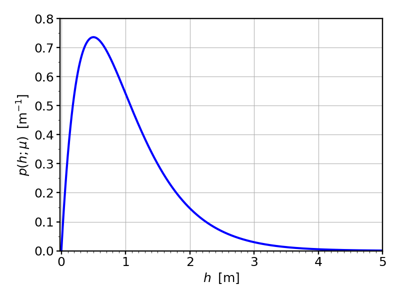
What’s plotted here is the probability density for water rising to a given (maximum) height $h$ on a given day. Before we go any further, it’s very important to understand how to read this curve. And how not to read it. In particular, the vertical axis is not a probability! For instance, the numerical value at $h=1\,{\rm m}$ is about 0.54, but this does not mean that the probability of that water height is 54%. Observe that the vertical axis has units, inverse meter, and this clearly shows that something different must be going on here. But even if we were to “overlook” that, we’d still run into problems when we discover that the numerical value at $h=0.5\,{\rm m}$ is about 0.74, and if we read this as 74%, then the aggregate probability of finding either one of the (mutually exclusive!) events $h=1\,{\rm m}$ or $h=0.5\,{\rm m}$ is 54% + 74% = 128%, which is more than 100% and hence makes no sense as a probability.

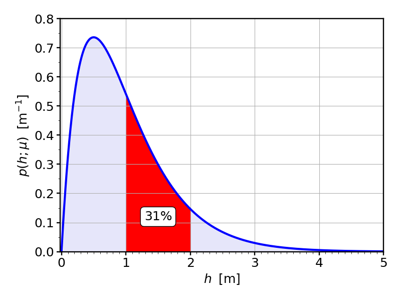
The correct way to interpret probability densities is to say that probability is hidden in the area under the curve. We have to ask questions such as: “what is the probability of the water level being between $h=1\,{\rm m}$ and $h=2\,{\rm m}$?” The area under the curve is the answer to that question. (Since the horizontal axis has units “meter”, and the vertical axis has units of “inverse meter”, the area becomes dimensionless, as it should for a probability!) Here, we find that this area is about 31% of the total area (which conventionally is just “normalized” to be 1), and so the chance of the largest water level on a given day being between one and two meter is 31%:

Since we want to do some calculations, it’s helpful to have some mathematical expressions for these probability densities. The one we have been using so far can be written as follows:

$$p(h;\mu) \;=\; \frac{4h}{\mu^2}\,{\rm e}^{-2h/\mu} \ , $$

Where $h$ is the water height and $\mu$ is a parameter that actually just denotes the average water height. (This happens to be a so-called “Gamma-distribution”, but the particular form really doesn’t matter that much.) In the above example we have chosen $\mu=1\,{\rm m}$, meaning that on average the water height is one meter. (If you’re wondering why that is not at the peak of the curve, observe that the curve is asymmetric and drags a bit to the right. And because of that, the average value need not coincide with the point where the density has its largest value.)

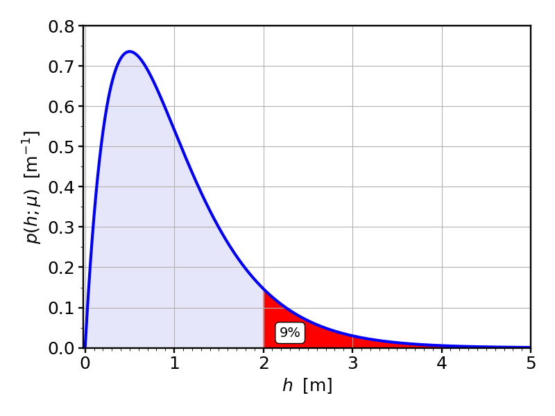
So far, so good. Now let’s get to the important question: recall that we want to build a levee that protects us from floods. What is the probability that the levee will fail to do that? Given what we’ve learned about area, it seems what we need is the area under the curve that’s to the right of some height $L$, the height of the levee. For instance, if we build a levee that’s at $L=2\,{\rm m}$, then we need to work out the following area:

Since we actually have a mathematical expression, we can do this with calculus. Don’t worry if you don’t know how that works. But you will have to trust me that I got the math right. The answer is:

$$\begin{align}P(h>L) \;&=\; \int_L^\infty{\rm d}h\;p(h;\mu) \\[1em] \;&=\;\left(\frac{2L}{\mu}+1\right)\;{\rm e}^{-2L/\mu} \ . \end{align}$$

If we plug in $\mu=1\,{\rm m}$, as in the figures, and pick $L=2\,{\rm m}$, we find a flooding probability of $0.0916\approx 1/10.92$, which means that the levee will flood about once every 11 days. Obviously not a good levee!

But now that we know how likely it is that the ocean will spill over the levee, given the levee height, we can set a goal. So let’s say the coast dwellers have debated the issue and decided that they want the levee to be such that it’ll be flooded only once every 500 years. That’s a very rare thing. Psychologically, this feels a bit like “never”, in the sense that neither we, nor our children, nor likely our grandchildren will ever experience such an event. But, of course, at some point disaster will strike. Just hopefully not for you!

So how high does the levee have to be for that to be true? Answer: we need to take the general formula for the flooding probability we have worked out above and set it equal to the super small probability the coast dwellers have agreed on. This gives:

$$\begin{align}P(h>L) \;&=\;\left(\frac{2L}{\mu}+1\right)\;{\rm e}^{-2L/\mu}\\ \;&=\; \frac{1}{500\times 365}\\[1em] \;&\approx \; 0.00000548 \ . \end{align}$$

We now have to solve this equation for $L$, which in truth is the only hard part, because this is a so-called transcendental equation, which we cannot solve in terms of simple inverse functions (such as roots or logarithms). But of course we can do this numerically, and then we find

$$\frac{L}{\mu} \;\approx\; 7.44 \ . $$

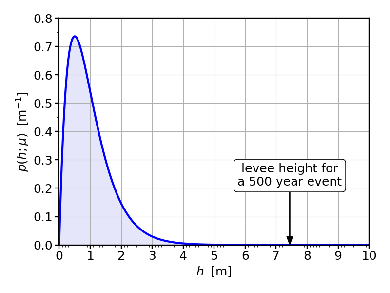
So if $\mu=1\,{\rm m}$, that means we need to make the levee $7.44\,{\rm m}$ high (24 feet and 5 inches). That’s quite a levee! Looking at the following picture of our probability density, we begin to appreciate how far into the very unlikely territory we need to go. It doesn’t seem like the water level would ever get to that point. The curve seems zero there! But it isn’t. After all, we are talking about rare events. That’s the whole point!

Now we come to the strange part. (Finally! Thanks for sticking with me this far!) We will look into the very counterintuitive behavior of the extreme event probability if something changes about our probability density.

Let’s say scientists predict that due to global warming the ocean level will rise by about $20\,{\rm cm}$ (about 8 inches). If you’re skeptical about global warming (which you should not, but that’s a different blog post), just imagine some other phenomenon that could affect water height, or simply remember that there are lots of other rare things that humans try to protect themselves against, and the same reasoning always applies. The key point I wish to get across is the following: if you’re standing at the coastline, admiring this veritable levee rising $6.44\,{\rm m}$ above the mean water height, you’d be forgiven to think that a $20\,{\rm cm}$ change in average water level is nothing compared to this impressive structure. The levee is 32 times higher than the predicted change in average water height. It will still be $6.24\,{\rm m}$ (20 ft, 5 in) higher than the average water level after the sea level rise has kicked in. It is absolutely natural to ask: why worry?

The answer is that we are not at all interested in average water heights! The levee has not been built to protect us against the average water height. It would be ludicrously over-designed for that purpose. It has been designed to protect us against a rare event, specifically one that we have previously all agreed on: a 500 year flood. The really interesting question is: with the average water level rising, what happens to the probability of the water level spilling over our levee?

Let us assume our mathematical model still works, but that we of course need to adjust its parameters. Specifically, the numerical value of the parameter $\mu$, which indicates the average water height, needs to change from $\mu=1\,{\rm m}$ to $\mu=1.2\,{\rm m}$. If we do this, then the new probability density for water height (plotted in green, and for comparison also the old one, still in blue) looks like this:

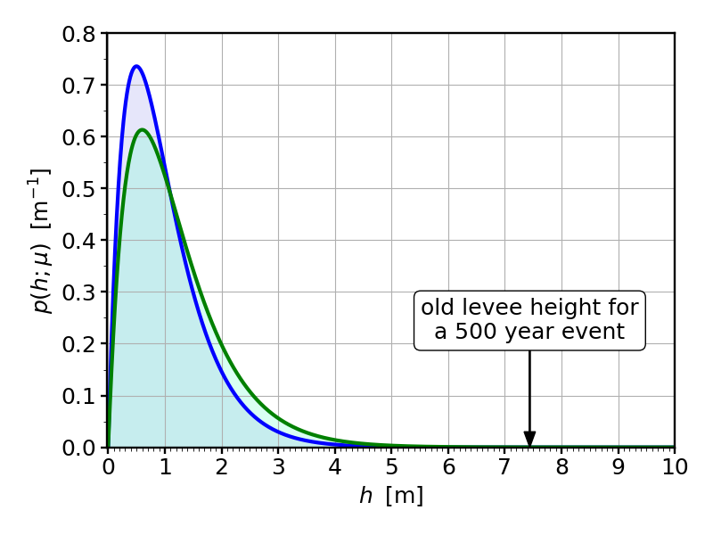
There are some obvious changes for low water heights, but it’s hard to see what happens in the “danger zone”: both curves are pretty much zero there. But be careful, we’re talking rare events, and what looks indistinguishable from zero on this plot is not really zero. In fact, we can simply calculate the spill-over probability, by inserting the value of the old levee height into the spill-over formula in which we replaced $\mu$ by its new value. We then find:

$$\begin{align}P_{\rm new}(h>L_{\rm old}) \;&=\;\left(\frac{2L_{\rm old}}{\mu_{\rm new}}+1\right)\;{\rm e}^{-2L_{\rm old}/\mu_{\rm new}}\\[1em] \;&\approx \; 0.0000552\\[1em]\;&\approx\; \frac{1}{50\times 365} \ . \end{align}$$

This should come as a huge surprise. The probability of flooding has increased (of course), but by a lot. Instead of it being a once in 500 years event, it’s now a once in 50 years event. That means chances are substantial that you will witness it in your lifetime.

It’s this extraordinary sensitivity of rare events to small shifts in the mean that makes reasoning about them so counterintuitive, and makes it so difficult to explain proper countermeasures to people unfamiliar with this fact. Nobody would just guess that a 20% increase in the mean leads to a 1000% increase in flooding probability. That just looks insane, but unfortunately that’s how rare event statistics often pans out.

So what should our coast dwellers do? Of course they still want to guard themselves against disaster, and let’s say that the “500 year flood” remains the acceptable worst-case scenario. Evidently, they must increase the height of the levee, but by how much? Looking at the equation we have used to calculate the levee height in the first place, we recognize that $L$ and $\mu$ only occur as a ratio, and that means if $\mu$ goes up by 20%, $L$ must go up by the same amount. Hence, the new levee should be $1.2\times 7.44\,{\rm m}=8.93\,{\rm m}$. That’s about one and a half meter higher than it was, more than 7 times the amount by which the average water height increased! So the counter measures are also much more involved than what we might naively expect based on the change of the mean:

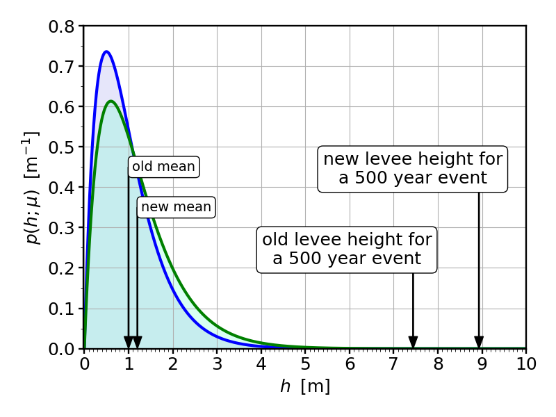
So there you have it. That’s today’s story about the extraordinary sensitivity of rare events on small changes of the mean. It is the main reason why we worry about changes in the water level due to global warming, or for that matter any changes of the mean values of our climate system. Consequently, the one thing that the Intergovernmental Panel on Climate Change (IPCC) is most confident about is the increased frequency of rare events—flooding, droughts, tornados, hurricanes, etc.

Intuitively, this effect is hard to grasp, and even many scientists are at times surprised when they encounter it in an unfamiliar setting. But it is really widespread—even in daily life! Have you ever wondered why we can fry a steak at 220C (approximately 430F), even though this temperature is only about 70% larger than room temperature (in Kelvin!), and the energy needed for breaking chemical bonds (say, for the Maillard reaction that colors the steak nice and brown) is many times larger than the thermal energy available even at frying temperatures? Answer: These chemical reactions are triggered by the extremely rare events in the tail of the so-called “Maxwell-Boltzmann” distribution, which describes the kinetic energy of the molecules. And by increasing the mean temperature by 70%, the probability of these rare events goes up millionfold. That’s in fact true for all temperature-triggered chemical reactions: they happen in the tail of the molecules’ kinetic energy distribution and are hence very sensitive to temperature changes!

So, the next time you encounter someone who is worried about the increased likelihood of rare events due to seemingly harmless changes of average values—now you know what’s afoot!

Markus Deserno is a professor in the Department of Physics at Carnegie Mellon University. His field of study is theoretical and computational biophysics, with a focus on lipid membranes.